There are no truly random numbers on a computer without special hardware. If it were any different, you would most likely complain that your machine is broken, since random behaviour is kind of the opposite of a computer’s intrinsically deterministic nature. Yet random numbers are in high demand for various purposes such as cryptography applications, statistical sampling, games as well as modelling and simulation. Understanding the difference between apparent and true randomness in practice is key to accomplishing those tasks.
The “Random String Generator” is a simple JavaScript tool designed to generate random strings and passwords based on the JavaScript engine’s internal random number generator plus some custom added salt. This article explains some of the mathematical and practical considerations that are interesting in the context of randomness.
The tool safely generates the random numbers on your computer, nothing of the generated random content is being transmitted to and from the server. Good for everyday use and most certainly better than some cooked up quick & dirty solution.
Two apparently random examples
Let us start with a simple, yet effective example. Consider the following two apparently random text blocks, each of which is a base-64 encoded1 file of originally 802 bytes of data:
iVBORw0KGgoAAAANSUhEUgAAAMgAAAClAQMAAAAj/CBZAAAABlBMVEX///8AAABVwtN+AAAAAXRSTlMAQObYZgAAAspJREFUeF7t1jGL1EAUB/A3N5JsMWa3nCK4K36BLAfHCMfdfpSIjYVgxMZCcI4DbQ79AjZ+A7+Bb1mwOqwtRy1sLBZsrjhc2clLnGTyOD3wtPAVO7C/ycvLZPmz8BdqysohclI6TrBgQFhe9B8RaTmZOiy6YkhMRRI9T2X6UpGUuieVawRIohNFujwuhM2aE3xkQ5jYn7KHkdAE+2UsNHUk7ZMuIqHTmeOgTB3XLbV2NouEajQsEwA13K0ASHFQZgACOIFhKS8hC1bwElKvibDpuiuilcxwolVPoJWMk6I/wUWSblqZ1iIBSU4aOSSxSN3eNlK5WrCR1yQCTU+OTOIlhbyWspFjrfRWMkhrqRp5oXK/2YBAL0V7zfjMb3b0MqVuRBw7gXU8GC+5FzraCvxN/AHeUo3cBL85p1gRn5NGdrebjaoA/Ajj47QRBQA7Ri0AfNfHUiIEta/8koNEKTpyUEsKN6Ane7VIG0XEbi3wxQLApCMndL8t61DmXmj7KJTiNBDVka+BJB25H2SC7Mj+L4mwoeSBAIaiQllAVCQlK0Un+kPRrIxYUawkrMhLiLCcLFlZASPiGSfyGic7ipNEc6IKTjQrk5KTAjkpLSdLVlYwJP3DAdlI/3Bg3Ej/cOA2iaaP+L/B0+iHiFW9rlxPUnFOgzyBbuXyuZfMjxKWySRSLq6lxUCcAUe5eNARaR0YSrF0hYGMBfo89Hn6zQWSp/W3eZjXvqq87mQolVs4W5gt48x5Ma3I734w7ebWi24lTet34ArwolpJZObXNUnWihKvvJyRJIFYLx9IZCSnkWhKoPckIpJ3JBB1W7VxE8kbTpZRvicUDBiJfMmJOCep+gIzuKCSf0L+y9XUdGnLYTEfOSkfcoJzVsRvi0CxccNixeYT2+2B5eQeslMPi2OlumPv2kE5XHLdxkd2sQCuWNGsXEdOUrjy+gG3Q/8jWFYdOgAAAABJRU5ErkJggg==
7InEUivzhs8KAdAoiAye7rspb87xgbE4hohXCv9ZGfRHRxQLW98FL0KCmMUDN4luLZ2/DFKeqzD3z8WFLbUHads1VlFheoiEzhrvKbXJSIK87TDdCienGqSYBWAZqOoDHDLFVnBGKw52qwHFKSg8JISGHLT4Gy5w2GExtLVoHhlroatEUhIjVXAVRNA47zR9/oFo5dkWtYaBSdWYeWJLSJC8fVlqDgb8T1eCfEJbbuS0MUXoEwlmchb915wixM5tlVs9wVGrneZsT2ZPTNjPhKL0Cs50b4oOynHKlnH/78xJttO53yBc2Or0d4FYSQ5zNUkxoucjZ+je1KBOlZSAMk1wV2nnECnvtCzjAWUfkWEjWVa5qjoVIPLopO+yc9FQG73gXJD4Agsqp1qcsw+ASktxRWlOJZg7oMKXU72Jyai/pKwgqQTYTgfLAYzs5qEvnXpgB9KmZpcy9h/4n9VyJbY1xOXGbB1zduXq5h9VIGQ5Qchcp6RaxIClpeWif7RJMPKwozUE4enjjPGtpTIEroMYvpVMulGTIGkGAKan+UEV4Hw6TwBjg3RlCpp8Ii3dF8wkHN0QjsmGQqEjrAjXZb3JvXSdb5TsR9SJu7CziV+MUuNjXOVry5ZhzB+Yf+dPpv1obaoRNsk5Gjydaj7eIUw9Ng66Nj+SpC+S7C/wxIri/v/2hX9jbWfFdE0z29AYciHZTvIcojchGSkAB+/RoqEuIWU9CF/GoVB7xLC9WJzhF3+o6Iggq+NQ+hWmetYT+K5Gg9Y50S7d0StIAclLYcM32YeOnMe3PfOZeHbAupf1QSRbTW9PPy/ZjmHo+xqgVffh4rZ0fg8EL+0/sKQTz/60EW/CpyxHe568yjPrPF80RiIxiJ7UaAwRxI6hU4patAY9+LPNDMGlV6n6Ct1Gi2hmpAVYznujotuEeLskn17Hm1hWjhlQPgPOsEieHgvmTGu0h/v67qi9b5xtfcpgMbrHGIxgDpPBS3w3r3ngP2Ct4Ehj3EYuggMIVxDFt2dfj5U6Apix7rN9Sct2PEwB0/EEeZfxbDgF90+EyzGb+qCLQg==
The majority of the two text blocks just looks like a completely garbled up sequence of letters and numbers. However, the beginning of the first text block might give you a hint: the somewhat out of place looking sequences of the letter A appear to be odd in comparison to the rest of text block. 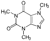 In fact, the first text block is a base-64 representation of a PNG image file, a highly compressed lossless file format, that shows the structure of the lovely molecule caffeine seen on the right.
The second text block, on the other hand, is indeed the base-64 encoding of a random file. But aside from the suspicious file header, which leads to the aforementionend sequences in the first text, there is little to distinguish the random file from some content, that has quite a lot of structure, i.e. an image. If the first 90 characters of both texts were cut out, it would be virtually impossible to distinguish both without a much deeper analysis. A simple statistical analysis like counting characters2 will reveal little, thus more advanced methods have to be applied. As we shall see lateron, compressibility and randomness are highly related concepts. We are therefore faced with the question, how true randomness can be characterized and distinguished from apparent randomness. In fact, this is a rather tricky issue and not at all obvious.
What is true randomness?
No one really knows for sure. From a mathematical perspective, true randomness is a somewhat hard to define and yet apparently intuitive concept. Before we dive into some of the mathematics relevant to understand randomness, let us briefly diverge to a more “physical” perspective on the topic at hand. Whereas the majority of scientists really believe in the existence of true randomness, in reality almost all experiments and observations are pseudo-random at best. The things and events that we normally call random are usually not at all random, but only appear to be so. Their apparent randomness is nothing else that a reflection of our ignorance about the thing or event that is being observed.
Imagine a coin flip for example: if you know every little detail of the coin, i.e. the precise mass distribution due to the engraving, the exact force being applied during the flip, the air pressure, temperature, humidity and all the minor little details of the surrounding environment, you would be very much able to predict the outcome of the coin flip. But in practice it is rather impossible to measure all those variables to the necessary amount of detail, which leads to the apparent randomness of the coin flip. Events we call random can therefore be classified as events where the number of external variables cannot be controlled precisely due to our level of ignorance.
A fundamental level of ignorance
However, there are events that to the best of our current understanding appear to be truly random. Radioactive decay would be one of those events. Given a macroscopic piece of radioactive material (say a kilo of uranium3), the average level of radiation and the exponential decrease in radioactivity due to decay of the material can be described very precisely. But we have absolutely no way of determining at which moment an individual uranium nucleus is going to decay—not a single hint. There is no “magic formula” to compute the precise decay event time of a given nucleus given all the external information of the environment. The best we can do is to compute something like the probability, that the nucleus will decay within the next 5 minutes or so. But knowing that the nucleus will decay with 99.999% probability (i.e. almost certainly going to decay) within the next 5 minutes tells you absolutely nothing about the moment of decay and whether or not the event is actually going to happen.
While the statistical properties describing radioactivity can be computed very precisely using quantum mechanics, the inherently probabilistic nature of the theory becomes very much apparent in such considerations. In order to compute the precise moment of a radioactive decay, we would require some additional input, something like a “hidden variable” describing some sort of a trigger. However, as shown by John Bell in 1964, according to the mathematical concepts underlying quantum mechanics, such a “hidden variable theory” would lead to fundamental inconsistencies.
One could of course argue that quantum mechanics is not the final arbiter of truth regarding microscopic phenomena. Just like Newtonian mechanics from the 17th century had been superseded by Einstein’s theory of general relativity, one could envision a future scenario where quantum mechanics has been replaced by some deeper theory. However, Newtonian dynamics reappears as a “low energy” solution to Einstein’s equations, thus the old theory is kind of embedded in the deeper theory. It is not wrong, it just fails to describe certain phenomena properly, when scenarios outside its original domain are considered. However, those shortcomings were already known during Newton’s time, since the shift of Mercury’s perihelion cannot be explained by Newtonian dynamics. One of Einstein’s big successes was it to finally solve the mystery and to provide an explanation.
This is not the case when it comes to quantum mechanics. Up to this point, there is not a single known experiment contradicting quantum mechanics. In fact, quantum electrodynamics—which builds on the fundamental of quantum mechanics—is the most precisely verified theory describing a part of our physical reality known to man. Therefore, any hypothetical theory that supersedes quantum mechanics at a fundamental level necessarily has to reduce to quantum mechanics for all experiments that at this point are known, which implies the same fundamental properties and limitations that have been derived from quantum mechanics. It is virtually impossible to imagine such a “quantum mechanics 2.0”, which on the one hand has to reduce to all experiments proving quantum mechanics as we know it, while on the other hand providing some apparently “deeper” understanding of nature.4
Therefore, if we take quantum mechanics for granted—and again, there is not a single experiment contradicting quantum mechanics—then we are forced to accept, that there are things in nature that we cannot know, i.e. a fundamental level of ignorance. For example, according to the Heisenberg uncertainty principle, one cannot measure the velocity \(v\) and position \(x\) of an elementary particle at the same time at arbitrary precision. The uncertainty \(\Delta x\) and \(\Delta v\) in both measurements is bounded from below, i.e. \[ \Delta x \cdot \Delta v \ge \frac{\hbar}{2}. \] Since this article should not turn entirely into a physics discussion, we summarize and (to the best of our knowledge) acknowledge that there are things in nature, which we cannot fully understand to the required level of precision. Thus, the universe has an inherent probabilistic nature and in the end this means that there are truly random events from our limited perspective. Radioactive decay is one of those events, so you better get hold of some uranium to improve your random numbers. Just put a Geiger counter next to some radioactive source and use the decay events as a source of randomness—done!
Hardware random number generators
Fortunately, radioactivity is not the only good source of randomness. Any other input, that is subject to our blissful ignorance of the precise variables of the event, is equally well suited to serve as a true randomness source in everyday applications. For example, thermal or static noise, electromagnetic noise or any other microscopic phenomenon that generates some sort of statistically random noise signals is good. If you dive deeper into the details, you will find that basically two types of physical phenomena are distinguished: those with quantum-random properties (like our radiactive decay example) and those without quantum-random properties (e.g. thermal noise). In the light of our previous discussion, sources using quantum-random properties appear to be better suited due to their dependance on a phenomenon that to the best of our knowledge cannot be fully known in its state. Yet, in everyday applications there is virtually no difference to good non-quantum-random sources, provided that the sampled environment variables are essentially not reproduceable.
It is unfortunately very easy to built hardware that produces a bad level of randomness. Considering the discrete nature of information in a computer, any such device that produces randomness, in the end has to provide a stream of randomly distributed bits, i.e. 1s and 0s with should be equally distributed. This means that the probability for a 1 and 0 should be 50% each, i.e. \(P(X=1)= P(X=0) = 0.5\).
Consider the discussed radioactive decay again as a direct randomness source: It is very well known, that a radioactive material has an exponential decrease in activity over time. If we simply take a Geiger counter and produce a stream of 0s and only a 1 when it clicks, the randomness distribution will be directly dependent on the sampling clock, which checks for a click and produces the 1 in case of an event. Over time, the radioactivity reduces and there will be (on average) more time between two clicks, which ultimately leads to a stream of a lot of 0s and only a few sparsely distributed 1s. While this stream is technically still truly random due to its source, the distribution of 1s and 0s will strongly diverge from the ideal 50:50 ratio. It is therefore necessary to either change the design of the machine (e.g. slow down the clock analogous to the expected exponential slowdown of the click amout per time), or to simply use the produced clicks in a different manner. Instead of using a “true” randomness source directly for the generation of 0s and 1s, it is often much more helpful to use a pseudo-random number generator and spice it up with some truly random input.
Pseudo-random numbers
A computer is essentially a Turing machine, which is a deterministic device that follows a specified series of instructions without any probabilistic properties. Therefore, a computer is in principle the worst kind of device to generate any kind of randomness. Nevertheless, random numbers most of the time originate from a computer, using a pseudo-random number generator (PRNG). Such a PRNG is nothing else than a mathematical prescription, that produces a series of seemingly random numbers from a given initial arbitrary seed state. However, other than a true random number generator, the produces series can be exactly reproduced given the initial state. Furthermore, due to the limited amount of data that the PRNG can use internally to represent its current state, every PRNG has a period after which the series of numbers is repeated. From a purely theoretical point of view, if the internal state is represented by \(n\) bits, the period can be no longer than \(2^n\) generated pseudo-random numbers and usually it is significantly shorter.
Despite the theoretical limitations, high-quality PRNGs can produce bit sequences that are extremely uniformly distributed and have extremely long period lengths. In fact, it is a open mathematical question if the produced bit sequence of a high-quality PRNG can be distinguished from the bit sequence produced from a true random generator if the PRNG algorithm is unknown. Due to the extreme period length one may be unable to identify any kind of correlation within the produced bit sequences. Nevertheless, designing good PRNGs that are suitable for cryptographic purposes—where the level of randomness is key to the security of the transported message—is a quite difficult task.
Various PRNGs have been constructed over the course of advances in cryptography. For a long time linear congruential PRNGs were the de-facto standard, which was later replaced by linear recurrence PRNGs. In 1997 the Mersenne Twister PRNG was discovered, whose period length in the most commonly implemented variant—called MT19937—is equal to the 24th Mersenne prime number \(2^{19937}-1 \approx 4.7\cdot 10^{6001}\), which in binary simply corresponds to 19937 times 1 in a row. It uses a standard word length of 32 bits and is \(k\)-distributed for \(k \le 623\), which means that it is not cryptographically secure as one can determine the algorithms internal state from a sequence of 624 produced pseudo-random numbers.5 A reference C code implementation is provided by the original authors, with various other implementations listed here. The Mersenne Twister is used by almost all languages and has found its way into the new C++11 standard, which is the reason it is specifically mentioned here. A decent explanation of its inner workings can be found on the corresponding Wikipedia page.
Mathematically defining randomness
We have reached a point, where we have a decent understanding of the difference between a true hardware-based random number generator and a pseudo-random number generator, which is basically just an algorithm that produces a cyclic sequence of apparently random numbers. Nevertheless, so far we have neglected to properly define randomness in mathematical terms and to provide a tool box to measure the level of randomness in a given sequence of numbers.
Randomness and entropy
One definition of randomness, found in a book by former IBM researcher Gregory Chaitin6 on the subject, states that “something is random if it is algorithmically incompressible or irreducible”. The random objects in a given set are those of the highest complexity, which is turn is related to their information content and entropy. If this rather abstract definition is applied to the specific case case of a finite series of bits or characters, this leads to the definition that a random string is one that is reasonably close to the highest possible complexity.
Before we can utilize this definition, we need to find a proper definition for complexity. The usual measure for the information content of a string—which is essentially equivalent to its complexity—is the Shannon entropy. Let \(s\) be a sequence of characters (i.e. a string) of length \(n\) and \(c=\{ c_1, ..., c_r \}\) be the list of unique characters used in the string. Furthermore, let \(k_i\) be the number of occurrences of the character \(c_i\) in the random string \(s\), then the Shannon entropy \(H(c,s)\) is defined by \[ H(c, s) = -\sum_{i=1}^r p_i \cdot \log_2(p_i), \qquad \text{where } p_i = \frac{k_i}{n} \] refers to the probability of the character \(c_i\) occuring in \(s\). The quantity \(H(c, s)\) describes the information content of a single character of the string \(s\), such that the total information content of the string \(s\) is given by \(H(s) = n\cdot H(c,s)\). In other words, \(H(s)\) gives the number of information carrying bits found in a string \(s\) of length \(n\).
Consider the implications of this definition for a moment: If a sequence of characters is just the same character over and over again, this definition implies, that the probability for a certain character is one and zero for all the other possible characters. Since \(\log_2(1) = 0\), the Shannon entropy of such a string would vanish completely, since a sequence of the same character over and over does not carry any intrinsic information at all. This may seem odd at first, since knowing which character is used over and over in the sequence and the number of repetitions of this character certainly counts as information as well. However, this kind of information is not intrinsic, as it depends on external knowledge like the alphabet from which the characters could be chosen. Other definitions of entropy exist, for example the Hartley entropy or Rényi entropy, but those will not be considered here.
Entropy measures the information content in a given string, i.e. the disorder or uncertainty that a characters appears. The entropy is therefore maximal, if the uncertainty of a character appearing is maximal. If an alphabet \(a= \{a_1,...,a_m\}\) of \(m\) characters is given, there are \(2^{n\cdot m}\) possible combinations to construct a string of length \(n\). In a perfect setting, an alphabet of length \(m\) implies that each letter carries \(\log_2(m)\) bits of information, such that the theoretical maximum information content of a string of length \(n\) is \(n \cdot \log_2(m)\) bits. This can be easily derived from the generic definition of the Shannon entropy above: in a perfectly random string each character appears with the same equally distributed probability \(p_i = \frac{1}{m}\), where \(m\) is the number of letters in the alphabet. Thus, we have \[ H(a,1) = -\sum_{i=1}^m \frac{1}{m} \log_2\left( \frac{1}{m} \right) = \frac{\log_2(m)}{m} \sum_{i=1}^m 1 = \log_2(m), \] which in turn implies \(H(a,n) = n\cdot H(a,1) = n \cdot \log_2(m)\). We refer to this maximum entropy of an \(n\)-string built from the characters in \(a\) by \(H(a,n)= n \cdot \log_2(m)\). If the string \(s\) is built from the alphabet \(a\), which implies that the unique characters \(c\) are a subset of the alphabet, i.e. \(c \subseteq a\), the definition of randomness can then be restated as follows: \[ \text{$n$-character string $s$ is random} \iff H(s) \approx \varrho(n) + H(a,n), \] where \(\varrho(n)\) describes a kind of string length dependent “cutoff value” up to whose value the string will be considered to be random. The statement essentially just formalizes, that the actual entropy of the given string should be reasonably close to the maximum entropy possible for such a string.
In addition to \(H(s)\), the normalized entropy or efficiency of a string \(s\) can be defined by the Shannon entropy \(H(s)\) divided by the logarithm of the string length \(n\). The resulting quantity \[ \eta(s) = -\sum_{i=1}^r \frac{p_i \cdot \log_2(p_i)}{\log_2(n)} = \frac{H(s)}{\log_2(n)} \] measures how equally distributed the unique characters are in the string independent of the string length. The normalized entropy is always in the range \(\eta(s)\in[0,1]\), where \(\eta(s)=1\) corresponds to a perfectly randomized (flat) distribution of the characters.
Storage and practical considerations
It is important to distinguish between the above computations of the entropy and the actual number of bits required to store the information. Given an alphabet \(a= \{a_1,...,a_m\}\) of \(m\) characters again, at least \(\lceil H(a,1) \rceil = \lceil \log_2(m) \rceil\) bits are needed for a direct representation of the alphabet, i.e. where each of the \(m\) unique characters is assigned the same bit sequence. A string of length \(n\) build from this alphabet therefore requires \(n \cdot \lceil \log_2(m) \rceil\) bits of storage capacity, even if its maximum information content is just \(\lceil n \cdot \log_2(m) \rceil\) bits. This is due to the fact that for each character \(2^{\lceil \log_2(m) \rceil} - 2^{\lfloor \log_2(m) \rfloor}\) of the combinations, that can be held in a \(\lceil \log_2(m) \rceil\)-bit sequence, are wasted if \(\log_2(m)\) is not an integer. Basically, if \(m\not= 2^j\) for some \(j\in\mathbb{N}\), for each character a fraction of a bit is wasted, which adds up to at most \(n-1\) bits in a string of \(n\) characters. Therefore, we have some bits wasted if the number of characters in the alphabet \(m\) is not a power of 2 simply due to representation issues.
You can test out the behaviour of all the defined quantities using the string entropy analyzer found on the random string generator page.
Randomness and representation
It is crucial to distinguish between randomness and representations in a different manner as well. If we apply the above considerations to our two initial examples—the base-64 encoded PNG image and the base-64 encoded random string—we find that both base-64 encoded strings show reasonably close values:
- The PNG image has a Shannon entropy of 5.89 bits/char and a normalized entropy of \(\eta = 0.5855\), which means that in the base-64 encoding the string contains 6319 bits of information of a theoretical maximum of 6456 bits, which leads to a 97.88% efficiency of the representation.
- The random string has a Shannon entropy of 5.97 bits/char and a normalized entropy of \(\eta = 0.5931\). Thus, the random string contains 6400 bits of information in base-64 encoding, and the theoretical maximum is 6456 bits, leading to a 99.13 % efficient representation. Storing the string at 7 bits/char requires 7504 bits.
This is not really surprising, considering that a PNG file is a highly compressed file format, i.e. we expect it to be close to the maximum entropy. However, a significant issue to consider is the fact, that the base-64 encoding itself potentially brings in a significant change of the entropy, since a different representation of the content may obfuscate structure. Consider the same random string in different encodings:
| String | entropy \(H(s)\) | \(\eta(s)\) | alphabet | entropy | max. bits | efficiency |
|---|---|---|---|---|---|---|
| random original | 7.78 bits/char | 0.8065 | 245 | 6214 | 6342 | 97.98 % |
| random base-64 | 5.97 bits/char | 0.593 | 65 | 6400 | 6456 | 99.13 % |
| random hex | 4 bits/char | 0.3753 | 16 | 6411 | 6416 | 99.92 % |
| random binary | 1 bit/char | 0.079 | 2 | 6415 | 6416 | 99,98 % |
As we can see, the efficiency does not vary much in different representations. This is not really surprising: considering that we took a random string, we are not expecting that there exists a representation in which an underlying structure of the string becomes apparent that could be used for an efficient storage. We would find the same result for the PNG file, since the PNG compression essentially transforms the original bitmap file to a high entropy compressed representation of the same data in a highly non-trivial fashion, which does not reveal itself by simply considering different character encodings.
Consider instead the well-known “Lorem ipsum” font and layout designer test text block and put it in different character representations.
Lorem ipsum dolor sit amet, consetetur sadipscing elitr, sed diam nonumy eirmod tempor invidunt ut labore et dolore magna aliquyam erat, sed diam voluptua. At vero eos et accusam et justo duo dolores et ea rebum. Stet clita kasd gubergren, no sea takimata sanctus est Lorem ipsum dolor sit amet. Lorem ipsum dolor sit amet, consetetur sadipscing elitr, sed diam nonumy eirmod tempor invidunt ut labore et dolore magna aliquyam erat, sed diam voluptua. At vero eos et accusam et justo duo dolores et ea rebum. Stet clita kasd gubergren, no sea takimata sanctus est Lorem ipsum dolor sit amet. Lorem ipsum dolor sit amet, consetetur sadipscing elitr, sed diam nonumy eirmod tempor invidunt ut labore et dolore magna aliquyam erat, sed diam voluptua. At vero eos et accusam et justo duo dolores et ea rebum.
| String | entropy \(H(s)\) | \(\eta(s)\) | alphabet | entropy | max. bits | efficiency |
|---|---|---|---|---|---|---|
| Lorem ipsum original | 4.1 bits/char | 0.4246 | 27 | 3295 | 3823 | 86.19 % |
| Lorem ipsum base-64 | 5.35 bits/char | 0.5312 | 53 | 5732 | 6141 | 93.34 % |
| Lorem ipsum hex | 3.29 bits/char | 0.3091 | 15 | 5295 | 6283 | 84.28 % |
| Lorem ipsum binary | 1 bit / char | 0.0787 | 2 | 6407 | 6432 | 99.61 % |
Due to the somewhat limited and repeated use of letters in the (seemingly) Latin language, we find that the original text block is not really a string of high entropy and far from random. In a base-64 encoding, it is much harder to pick up on this, but compared to our random example above, there is a significant deviation from a truly random string. The hexadecimal encoding strongly highlights the non-random structure of the underlying data again, which is not exactly surprising: from an 8-bit ASCII letter representation to 4-bit hexadecimal encoding, one essentially splits up each byte into two pieces. Thus, the redundancies found in the original text are more or less preserved. Only the binary representation, where any sort of information on the grouping of the 1s and 0s is technically completely lost shows a value somewhat comparable to the random data.
If we consider a longer English language text block those results are more pronounced. Even the binary encoding of the input shows a somewhat significant dip in \(\eta(s)\):
| String | entropy \(H(s)\) | \(\eta(s)\) | alphabet | entropy | max. bits | efficiency |
|---|---|---|---|---|---|---|
| Long text original | 4.45 bits/char | 0.312 | 66 | 86615 | 117769 | 73.55 % |
| Long text base-64 | 5.41 bits/char | 0.369 | 63 | 140582 | 155290 | 90.53 % |
| Long text hex | 3.33 bits/char | 0.2184 | 16 | 129803 | 155872 | 83.28 % |
| Long text binary | 0.99 bits/char | 0.0575 | 2 | 154690 | 155872 | 99.24 % |
Thus, we clearly see that the above definition of randomness does not really take the issue of representation into account. Unfortunately, for strings of finite length one can in theory always construct an efficient representation which will make the data look well organized. This prohibits the formal definition of a representation independent notion of a random string. We therefore have to keep in mind, that the interpretation of randomness is a representation dependent issue.
Implementation
After all those considerations let us come to the actual JavaScript random string generator implemented here. We are essentially faced with several problems: On the one hand, the random number generator that is used by the standard Math.random() JavaScript function is an unspecified detail of the specific implementation the web browser uses. Chances are good, that it uses the Mersenne twister algorithm. On the other hand, no detail on the initial seed value of the function are known. This is not exactly good, if we want to generate truly random numbers, which cannot be reproduced.
The idea is therefore to assume, that the Math.random() function only has a decent PRNG behaviour but cannot be trusted due to the unknown initializer, which means that is has a very long period but we do not know whether or not it is easy to reproduce the initial state. This means that we need to “salt” it using some external source of randomness. We therefore collect a sequence of mouse movements in the browser window and use the \((x,y)\) position information of the mouse cursor together with a time stamp of the recording moment to generate a random 128-bit number. This is used as an additional source of randomness to the build-in Math.random() pseudo-random number generator.
The 128-bit salt is represented by four 32-bit unsigned integer values. At each mouse movement event we basically shuffle around the four numbers, and mix in the position and time stamp information to update the 128-bit number. On a 1080p Full-HD screen, this gives us \(1920 \cdot 1080 = 2073600\) position combinations plus the time stamp plus the input from the build-in random number generator. We can therefore safely assume, that even after just a few mouse movements we have a created a purely random 128-bit number. Just to give you an idea: a 128-bit number has \(2^{128} \approx 3.4 \cdot 10^{38}\) possible combinations. In theory, six mouse position combinations would be enough to randomize the 128-bit salt. However, mouse movements are not equally distributed over the entire screen space, such that we collect significantly more positional information in order to ensure the salt is properly initialized. The updating of the random 128-bit “salt” is carried out by the following piece of JavaScript code:
var seedevents = 0;
var eventseed = [ ((new Date()).getTime()*41 ^ (Math.random() * Math.pow(2,32)))>>>0,
                  ((new Date()).getTime()*41 ^ (Math.random() * Math.pow(2,32)))>>>0,
                  ((new Date()).getTime()*41 ^ (Math.random() * Math.pow(2,32)))>>>0,
                  ((new Date()).getTime()*41 ^ (Math.random() * Math.pow(2,32)))>>>0 ];

function addRandomSeedEvent(e)
{
    seedevents++;
    eventseed[0] = ((eventseed[3] * 37)
                    ^ (new Date()).getTime() * 41
                    ^ Math.floor(Math.random() * Math.pow(2,32))
                    + (e.clientX||e.screenX||e.pageX||1)
                    + (e.clientY||e.screenY||e.pageY||1) * 17) >>> 0;
    eventseed[1] = ((eventseed[0] * 31)
                    ^ (new Date()).getTime() * 43
                    ^ Math.floor(Math.random() * Math.pow(2,32))
                    + (e.clientX||e.screenX||e.pageX||1)
                    + (e.clientY||e.screenY||e.pageY||1) * 19) >>> 0;
    eventseed[2] = ((eventseed[1] * 29)
                    ^ (new Date()).getTime() * 47
                    ^ Math.floor(Math.random() * Math.pow(2,32))
                    + (e.clientX||e.screenX||e.pageX||1)
                    + (e.clientY||e.screenY||e.pageY||1) * 23) >>> 0;
    eventseed[3] = ((eventseed[2] * 23)
                    ^ (new Date()).getTime() * 51
                    ^ Math.floor(Math.random() * Math.pow(2,32))
                    + (e.clientX||e.screenX||e.pageX||1)
                    + (e.clientY||e.screenY||e.pageY||1) * 29) >>> 0;

    // Update the output
    setTagContent('mmoveevents', seedevents);
    setTagContent('random-seed', '0x' + ('00000000' + eventseed[0].toString(16)).slice(-8)
                                      + ('00000000' + eventseed[1].toString(16)).slice(-8)
                                      + ('00000000' + eventseed[2].toString(16)).slice(-8)
                                      + ('00000000' + eventseed[3].toString(16)).slice(-8));
}
The JavaScript Math.random() function is then basically replaced by unsignedRandom(maxval, i), where i is an arbitrary number (e.g. a counter) and maxval is the maximum random integer value. The random string \(s\) is then constructed from a simple loop over the length \(n\), where the character set index is the random number:
function unsignedRandom(maxval, i)
{
    return Math.abs( (Math.floor(Math.random() * Math.pow(2,32))
                     ^ (eventseed[i % 4] >>> (i % 23)) )
                       % (maxval+1) );
}

function randomString(length, chars)
{
    var result = '';
    for (var i = length; i > 0; --i)
        result += chars[unsignedRandom(chars.length - 1, i)];
    return result;
}
Our generation of the random string is therefore based on randomly choosing a character from the alphabet, where the random index is constructed from the Math.random() function, and the collected 128-bit salt. We can therefore safely assume, that for the reasonably short string lengths produced by the random string generator, the strings are both random and not reproduceable, even if the JavaScript engine is using a weak or outdated PRNG implementation.
-
Base-64 encoding is used to represent binary data in text form. It splits up a group of three 8-bit bytes to a group of four 6-bit numbers, which can then be expressed in terms of normal letters. You may want to check out the Encoding Converter to get familiar with this type of encoding. ↩
-
Just for the fun of it, you can copy and paste the two base-64 encoded text blocks to the “string entropy analyzer” section found at the bottom of the random generator page. One somewhat significant difference between the two text blocks ist a much wider variance \(\chi^2 = 231.4\) of the character count for the PNG file compared to \(\chi^2 = 71.56\) of the random file. The two text blocks each have a length of \((267 + 1)\cdot 4 = 1072\) characters (four thirds of \(267 \cdot 3 + 1 = 802\) input characters plus padding). If you compare this to the \(\chi^2\) values typically found in the generated 1000 random alphanumeric characters, we find that the two values are reasonably close. This is not a surprise, considering that the base-64 encoding does not change the underlying randomness of the 802 random binary bytes. ↩
-
Despite all the rumors and myths surrounding the element uranium it is not extremely radioactive or dangerous. Whit it is probably not the best idea to eat it—extremely toxic: it accumulates in your kidneys where aside from alpha radiation its chemical properties are lethal—a chunk of natural or slightly enriched uranium is a good radiation source for lab experiments. The artificial radiactive elements are the truly dangerous ones due to their extreme levels of radiation. ↩
-
The reader might argue that we already know situations where quantum mechanics fails: black holes and other extreme situations where gravity and quantum mechanics are on an equal footing. However, it is not the probabilistic nature of quantum mechanics, that blows up at this point. It is our current mathematical formalism of quantum mechanics, which is based on a fixed “stage” incompatible with the dynamic nature of general relativity, that is the cause of all the problems. A unified theory of quantum gravity is expected to integrate the vastly different mathematical descriptions and concepts of both quantum mechanics and general relativity, but it has to reduce to both theory in the respective limit cases. In any case, for the discussion of randomness at hand, this does not change the essential insight that our limited ability to observe events is ultimately the origin of (apparent) randomness. This is the stuff for lengthy philosophical discussions… ↩
-
By no means does this imply that it is simple to reconstruct the internal state of the Mersenne Twister given such a sequence of 624 generated pseudo-random numbers. However, it is in principle possible and computationally feasible, which rules the algorithm out for cryptographic applications. ↩
-
See the book “Exploring RANDOMNESS” by Gregory J. Chaitin. ↩