In this article the loss of significance in floating-point computations is discussed and analyzed in C# and C/C++. Different implementations of the floating-point engine in hardware and software will be discussed. In the end, we are compiling a best practices guide in order to minimize the effect.
Floating-point arithmetic has been a source of both tremendous advances and terror alike. On the one hand it expands the value range of numbers available for computations considerably beyond integers, on the other hand one now has to deal with the issue of a loss of significance. In order to approach the subject we are going to discuss the elementary data types at first, introduce floating-point numbers and then investigate the loss of significance due to arithmetic operations.
Integer data types
Any binary machine in its most basic form is only able to understand… binary numbers. What a surprise! So we are dealing with ones and zeroes in the representation of any number on a computer, which are usually called bits. A single bit has only the two stable states 0b and 1b. Naturally, we are grouping together several bits in order to describe larger numbers: 1 byte consists of 8 bits, for example, and this gives us \(2^8=256\) possible combinations. If we identify the sequence of bits 00000000b with the numeric value of zero and build up from there, using standard base-2 addition, we can effective describe the integers 00000000b = 0d to 11111111b = 255d in one byte, where we use b to denote binary numbers and d to highlight (ordinary) decimal numbers. This approach generalizes to sequences of bits with arbitrary length and defines the notion of a unsigned integer.
Signed magnitude representation
Another possibility is to treat one of the bits in a byte differently. For example, we can interpret the very first bit as an indicator for the minus sign in an ordinary number. For simplicity, we would want to keep identifying 00000000b with the numeric value of zero and up to 01111111b = 127d everything remains the same. However, if we reach 10000000b we find a disambiguity. If the first bit corresponds directly to the minus sign and the remaining bits represent the actual number, this would be interpreted as -0d, which is mathematically equivalent to +0d. In our system, we would have 10000001b = -1d and 11111111b = -127d. So, in the end, we are left with an easily readable system to describe numbers in the range of -127d to 127d with only one small redundancy for the zero. Not too bad. In fact, some early binary computers around 1960 used this exact representation and it is still used in part for floating point numbers, as we will see below. In the end, this simple system is called the signed magnitude representation.
Two’s complement signed integer convention
Obviously, when something is too simple, it is no good in the real world. And wasting a single precious numeric state indeed has its drawbacks. Therefore, computer scientists in the early 1960s came up with three different methods to circumvent the redundancy arising from the “sign bit” in the signed magnitude representation, of which—fortunately—only a single one survived. Again, we define the bit-wise zero 00000000b to be equal to the decimal zero 0d in order to have a sane fixpoint. Likewise, from 00000001b = 1d up to 01111111b = 127d everything remains the same. But then for the very first bit we introduce a big shift by 256, which leads to 10000000b = -128d. If you ever wondered why adding to a signed positive integer may lead to a sudden change in the sign, then this is exactly the reason! From 10000000b = -128d we can now go up again, such that 10000001b = -127d to 11111111b = -1d fills up all the negative integers that we need to account for in a single byte.
The reason for the big shift between 01111111b = 127d and 10000000d = -128d is that the arithmetic of the binary addition is preserved. If we start with the smallest negative number, that we can describe in a signed byte, 10000000d = -128d, we can reach 11111111b = -1d by simply adding 00000001b = 1d in the usual fashion. Adding 11111111b + 00000001b = 1 00000000b then leads to a binary overflow, where the most significant bit is lost due to the limited size of the byte, but the remainder 00000000b = 0d corresponds to the correct result. And that is ultimately the reason for this decision of representing signed integers: we can preserve the behavior of binary addition when crossing from negative to positive numbers (and vice versa). In the end, this choice simplifies the electrical circuit design for the adder significantly. One has to remember that a lot of those fundamental choices were made at a time, where instead of billions of transistors inside a small piece of silicon, discrete electron tubes and manually wired connections were used.
This system of describing negative integers, which is called the “two’s complement” convention, naturally extends beyond an 8-bit byte to arbitrarily sized integers. This leads to the following ranges of integers of different capacities:
| size | signed minimum value | signed maximum value | unsigned maximum value |
|---|---|---|---|
| 8-bit | -128 | 127 | 256 |
| 11-bit | -1,024 | 1,023 | 2,048 |
| 16-bit | -32,768 | 32,767 | 65,536 |
| 23-bit | -4,194,304 | 4,194,304 | 8,388,608 |
| 32-bit | -2,147,483,648 | 2,147,483,647 | 4,294,967,296 |
| 52-bit | -2,251,799,813,685,248 | 2,251,799,813,685,247 | 4,503,599,627,370,496 |
| 64-bit | -9,223,372,036,854,775,808 | 9,223,372,036,854,775,807 | 18,446,744,073,709,551,616 |
Fixed-point numbers
While integers are a useful and natural representation of numbers, one sooner or later arrives at a point, where real numbers and fractions of an integer are required. The simplest way to approach this issue is to use fixed-point numerics, which implies that we treat a certain number of digits as the fractional digits following the point. In a decimal notation, for example, we can take the last 6 decimal digits and declare them to be “after the point”, which means that we impose an implicit factor \(10^6\) when representing our number as an integer. For example, we treat the integer 73322554d as the decimal fraction 73.322554d. Using this approach we do not even have to change the definition of an addition, because two numbers with a common shifting factor can simply be added up and everything works as before. Even multiplication remains simple: we just multiply the result like regular but then have to divide it by the common factor, which essentially discards the least significant digits after the point. We only have to be careful with regard to overflows, but such things can be properly considered and are being dealt with. The same principle can also be applied to the digits in a different number base, for example in base-2, which just means that a certain number of bits are considered to be “behind the point”. Fixed-points numbers are therefore very simple and can be reasonably efficient implemented. They are often used in financial contexts where rounding errors and a loss of significance have to be avoided. Nevertheless, depending on the chosen implicit shifting factor, one either quickly looses on precision for small numbers or is severely constrained in the largest possible values.
Floating-point numbers
Scientific notation and base-2
This is where floating-point numbers come in: instead of a fixed implicit factor, the factor itself becomes part of the number, which in effect allows it to vary for each number individually. Basically, we are writing the number in an (almost-)scientific notation like
\[
-423745.6458832 = -4.237456458832 \cdot 10^6,
\]
where 4.237456458832 is called the mantissa and 6 the exponent. Instead of using a decimal fraction, we can also use any other number base, so once again binary or base-2 looks good in the context of representing a number on a computer. With respect to base-2 the mantissa is always contained within the interval \([1,2]\). For efficiency reason, the most significant bit of the mantissa, which is always a 1 since it determines the exponent value uniquely, is omitted.
To summarize: We have an overall sign indicator bit \(\sigma\), a mantissa \(m\) that represents a number in \([1,2]\) and a signed integer exponent \(e\). Any number \(x\) can then be represented by \[ x = (-1)^\sigma \cdot m \cdot 2^e, \] which is a minimal deviation from the scientific notation. Those three elements are all that make up a floating point number, which is is arranged as follows in case of a 64-bit floating-point number:
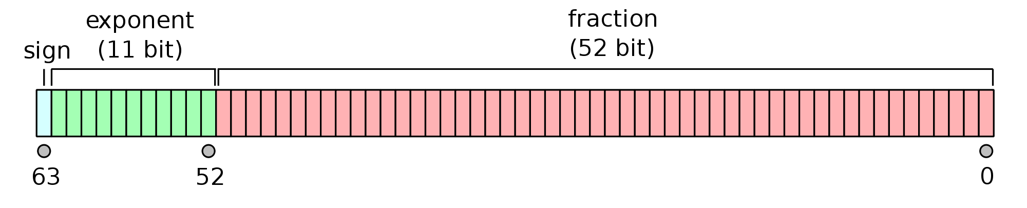
Since a double-precision floating point has 11 bits for the signed integer exponent, we can represent the range from -1022 up to 1023, which—considering that we use this exponent for a base-2 number—means we can descibe numbers up to \(2^{1023} \approx 10^{308}\). This follows from the exponent conversion factor \(\log_{10}(2)\approx 0.301\) or \(\log_2(10)\approx 3.322\).
How can we operate with those numbers? A floating-point multiplication is deceptively simple: We just multiply the two mantissa, which gives us the new mantissa, and we add up the two exponents—done! For an addition we have to work a little bit harder. Essentially, the larger exponent determines the overall exponent, so we shift the mantissa of the number with the smaller exponent until we have both numbers on the same exponents and then we add up the mantissa. After some normalization and bringing the number back into the standard format, we have the sum of the two floating-point numbers.
Floating-point numbers have truly a long history. Zuse’s Z3 machine already used 22-bit floating-point numbers and various other variants have been used in the early decades of computers. Nowadays, only the single and double precision floating point numbers (32 and 64 bit, respectively) are used on standard computers.
Floating-point numbers by the bits
The obvious drawback of floating-point numbers is the fact that the precision of the represented number is limited by the size of the mantissa. Before we can do anything substantial to investigate the loss of significance problem, we need an easy way to look at the bits of our computations. Therefore we use the following piece of C# code:
using System;

namespace BinaryFP
{
    class Program
    {
        public static unsafe string GetDoubleBits(double value)
        {
            // Convert the 64-bit double floating-point to 64-bit integer
            long num = *((long*)&value);
            // Use the build-in method to convert to base 2
            return Convert.ToString((long)num, 2).PadLeft(64, '0');
        }

        public static string GetDoubleBitsNiceFormat(double value)
        {
            string bits = GetDoubleBits(value);
            return String.Format("{0:0.0000} d  =  {1} {2} {3} b", value,
                bits.Substring(0, 1), bits.Substring(1, 11), bits.Substring(12)).PadLeft(82);
        }

        static void Main(string[] args)
        {
            Console.WriteLine(" decimal    sign  exponent                         mantissa");
            Console.WriteLine(GetDoubleBitsNiceFormat(-1.0));

               // ...well, all the numbers one would like to digitize...

            Console.WriteLine(GetDoubleBitsNiceFormat(Math.PI-2.0));
        }
    }
}
Using the simple quick and dirty unsafe pointer hack *((long*)&value) to reinterpret the double as a long in order to obtain the bits from a double floating point number without a numeric conversion, we can split up the resulting 64 character string of 0s and 1s to highlight the sign bit, the exponent bits and the mantissa. Running the program then yields the following output:
 decimal    sign  exponent                         mantissa
-1.0000 d  =  1 01111111111 0000000000000000000000000000000000000000000000000000 b
 1.0000 d  =  0 01111111111 0000000000000000000000000000000000000000000000000000 b
 0.0000 d  =  0 00000000000 0000000000000000000000000000000000000000000000000000 b
We see the sign bit corresponding directly to the actual sign of the number, which fits in to the discussed signed magnitude representation and follows the \((-1)^\sigma\) portion of the scientific notation mentioned earlier.
The proper interpretation of the exponent is only slightly more complicated: for once, we observe that the value of zero—in this case represented by the decimal 0.0—is once again represented by a pure sequence of zero bits. It is a special value, which (slightly) violates the generic structure of the floating point interpretation. The exponent \(e\) is a signed integer, but it does not follow the “two’s complement” structure that was discussed. Instead, it is simply an unsigned integer that has been shifted by -1023d, such that the the exponent 00000000000b = 0d is interpreted as -1023d. This shift is called the excess-\(k\) signed integer representation, where \(k\) is the shift. For a 64-bit double precision floating-point number with an 11-bit wide exponent we are therefore dealing with an excess-1023 signed integer exponent. In particular, this implies that the unsigned sequence of bits 01111111111b = 1023d has to be read as the signed value 0d, and this leads to the correct interpretation of the bit sequence output for the number 1.0 on the listing above: it is to be read as \(1.0 = (-1)^0 \cdot 1.0 \cdot 2^0\), i.e. we find \(\sigma=0\) for the sign indicator, \(m=0\) for the mantissa and \(e=0\) for the exponent, which in the excess-1023 representation gives the bit sequence 01111111111b. This is exactly, what we are seeing in the output listing.
Examples
Let us consider a somewhat more difficult example. Whereas the integer representation of 11d = 00001011b is straightforward to obtain from \(11 = 8+2+1 = 2^3 + 2^1 + 2^0\), we need to rewrite this number as a base-2 fraction to obtain the floating-point representation. The most significant bits of the mantissa are to be treated as negative powers of 2, i.e. the first bit represents \(2^{-1}=0.5\), the second one \(2^{-2} = 0.25\), \(2^{-3} = 0.125\) and so on. Since we have \(2^3 = 8 \le 11 \le 16 = 2^4\), we know that \(\frac{11}{2^3} = 1.375 \in [1,2]\) is in the correct base-2 mantissa range, such that we find \(e=3\) for the exponent. Using the excess-1023 signed integer representation, this \(e=3\) corresponds to the bits 1026d = 10000000010b. In terms of the base-2 mantissa, we can then deduce that \(1.375 = 1 + 0.25 + 0.125 = 1+2^{-2}+2^{-3}\) represents the fraction, which—discarding the obvious leading value 1.0—leads us to the mantissa bits 0110000...b. A quick look at the output of our little C# program shows that the bit sequence of this is indeed correct:
-11.0000 d  =  1 10000000010 0110000000000000000000000000000000000000000000000000 b
 11.0000 d  =  0 10000000010 0110000000000000000000000000000000000000000000000000 b
For all positive and negative integers we find that this structure remains pretty much the same. Interesting things begin to happen, when we are considering fractions that have no direct integer correspondent. In the base-10 system numbers and fractions divisible by 2 and 5 can be accurately written as a decimal number. This is why \(\frac{1}{4}=0.25\) has a finite number of decimal fractions and \(\frac{1}{3}=0.333333...\) has an infinite period of 3s. In base-2 only numbers built from powers of 2 can be accurately represented, which leads to the following effects when we are representing the inverse integers \(\frac{1}{2}\), \(\frac{1}{3}\), … via double precision floating-point numbers:
1.0/2.0  =  0.5000 d  =  0 01111111110 0000000000000000000000000000000000000000000000000000 b
1.0/3.0  =  0.3333 d  =  0 01111111101 0101010101010101010101010101010101010101010101010101 b
1.0/4.0  =  0.2500 d  =  0 01111111101 0000000000000000000000000000000000000000000000000000 b
1.0/5.0  =  0.2000 d  =  0 01111111100 1001100110011001100110011001100110011001100110011010 b
1.0/6.0  =  0.1667 d  =  0 01111111100 0101010101010101010101010101010101010101010101010101 b
1.0/7.0  =  0.1429 d  =  0 01111111100 0010010010010010010010010010010010010010010010010010 b
1.0/8.0  =  0.1250 d  =  0 01111111100 0000000000000000000000000000000000000000000000000000 b
We can clearly make out the base-2 fractional periods for any numbers other than negative powers of two. Note that \(\frac{1}{3}\) and \(\frac{1}{6}\) share the same mantissa and only differ by 1 in the exponent. This follows directly from \(\frac{1}{6}=\frac{1}{3} \cdot \frac{1}{2} = \frac{1}{3} \cdot 2^{-1}\).
Special numbers and binary values
It was already mentioned that the floating-point number 0.0 is represented by the special sequence of zero bits 00...00b, that breaks the sign-exponent-mantissa representation somewhat—otherwise it would represent the number \((-1)^0\cdot 1.0 \cdot 2^{-1023}\approx 1.11\cdot 10^{-308}\). There are several other special numbers, that are important to know:
- Signed zero: According to the IEEE-754 standard for floating-point numbers, the number zero is signed, which means that there is both a positive \(+0.0\) and a negative \(-0.0\) value. Both are distinguished by the sign bit as usual, which is shown in the listing below.
- Signed infinity: Likewise, there are two infinite values \(+\infty\) and \(-\infty\), which are represented by the maximum exponent
11111111111band a zero mantissa. - Not-a-number (NaN): This value describes the result of an invalid operation like \(\frac{0}{0}\), \(\sqrt{-1}\) or other likewise ambiguous and/or mathematical ill-defined operations. It is represented by the maximum exponent
1111111111band a non-zero mantissa. In theory the entire 52 bits of a double precision floating-point mantissa could be used to encode the specific type of the NaN, but there is no official standard such that one usually only checks if the mantissa is non-zero.
The reason for including signed zero values and signed infinities is to properly represent the extended real number line \(\bar{\mathbb{R}} = \mathbb{R} \cup \{ +\infty, -\infty \}\). This allows to perform computations like \(\frac{1}{\pm 0.0} = \pm \infty\) and vice versa, which are both valid in this domain. In bit-wise representation we have the following bit sequences for the mentioned special cases of double precision floating-point numbers:
 decimal    sign  exponent                         mantissa
-0.0000 d  =  1 00000000000 0000000000000000000000000000000000000000000000000000 b
 0.0000 d  =  0 00000000000 0000000000000000000000000000000000000000000000000000 b
-infinity  =  1 11111111111 0000000000000000000000000000000000000000000000000000 b
 infinity  =  0 11111111111 0000000000000000000000000000000000000000000000000000 b
      NaN  =  1 11111111111 1000000000000000000000000000000000000000000000000000 b
Depending on the selected run-time mode of the floating-point engine, NaNs can be either silent or signaling, which means that an exception is thrown if an NaN is produced as the result of a mathematical operation.
Implementation history
The concept of floating point numbers goes back to the earliest instances of machines that are able to perform arithmetic computations. Once one has designed a binary adder circuit for the arithmetic manipulation of unsigned integers and implemented the rudiments of conditional program flow control, one can begin dealing with floating-point numbers. However, the necessary use of bit-masks to manipulate the sign, exponent and mantissa individually, the various operations of shifting the mantissa to align the exponents and so on require quite a number of separate operation steps if they are emulated on an integer-based computational machine.1 Therefore, in the old days floating-point operations were only used if circumstances prohibited other means of computation and the overhead was quite significant unless specialized hardware was used.2
All of this changed with the introduction of the (somewhat affordable) mathematical co-processor, which first appeared in the 1970s for early desktop computers. The famous Intel 8087 floating-point co-processor unit, called FPU, significantly expanded the available instruction set and led to speedups of a factor of around fifty in math heavy applications. Within the FPU, all the required individual integer operations that would emulate the floating-point operations, like addition and multiplication, are more or less hard-wired in the circuitry. Instead of a rather large number of integer operations on the CPU, the FPU can carry out the operation in a significantly fewer number of steps. With the introduction of the Intel 80486 generation of processors, the FPU became an integral part of the CPU and in todays modern processors floating-point operations can essentially be carried out almost as fast as integer operations. With billions of transistors available, all the potential situations and cases that can arise in a floating-point computation can simply be hard-wired, which effectively reduces the number of necessary computation steps.
An important choice in the design of the original x87 co-processor was the abnormal size of the FPU-internal registers: instead of 32-bit single precision or 64-bit double precision floating-point representations, the engineers opted for 80-bit wide FPU-internal computation registers. The idea was to provide additional bits for both the exponent and the mantissa, that are to be used in intermediate computations to minimize the unavoidable rounding errors and minimize the loss of significance. From today’s perspective this can be seen as a historical relic, since a number of those problems can be avoided using smarter hardware implementations, but the 80-bit extended FPU registers are still present in modern CPU-integrated FPUs. Some programming languages allow for a direct access to those extended data formats, for example the long double type in C/C++ (which is, however, implementation-dependent and may actually reduce to the standard double). We will have to keep the existence of such extended data formats in mind when we are going to analyze the loss of precision.
In fact, in modern desktop processors the classic x87 FPU has been superseded by more advanced extensions to speed up mathematical computations. During the late 1990s and early 2000s the computational requirements of modern 3d computer graphics and video processing lead to the introduction of the concept of parallel processing for mathematical operations. For example, in typical matrix-vector operations one performs the same mathematical operation multiple times on different numbers, such that the concept of SIMD (single instruction, multiple data) was introduced in a modern extension of the FPU. This essentially allows to perform the same mathematical operation on several floating-point numbers at the same time. With the inclusion of the SSE and SSE2 extensions in all x64 CPUs, the old x87 FPU has been depreciated and only remains for compatibility reasons to 32-bit legacy code. This is quite important: While the old x87 FPU allowed to make use of the internal 80-bit registers, the newer SSE2 registers are only holding 32-bit or 64-bit floating point numbers internally. At least in theory, the loss of significance and precision therefore was less of a problem on older machines with the classic FPU. However, in terms of performance SSE2 allows for significant advances, which in the end is a very useful trade-off.
The IEEE-754 floating-point standard also includes specifications for a 128-bit quadruple precision format, which back in the 1970s was envisioned to replace the 64-bit double precision format as soon as silicon would become cheap enough. However, except for special purpose chips, the 128-bit implementation never found any widespread adoption and—depending on the type of application—the 32-bit single and 64-bit double precision floating-point numbers are the only two types used in practice nowadays.
Mathematical operations and loss of significance
Addition and multiplication for floating-point numbers
In order to understand the origin of the “loss of significance” problem we are going to discuss the two most basic arithmetic operations on floating-point numbers: addition and multiplication. In fact, since binary multiplication reduces trivially to addition,3 we only need to consider the former one of the two. We are going to compare the effect on single and double precision floating-point numbers. Therefore, we expand out little C# program by the following two functions, which provide the same bit sequencing functionality for the 32-bit single precision float data type:
public static unsafe string GetFloatBits(float value)
{
    // Convert the 32-bit float floating-point to 32-bit integer
    int num = *((int*)&value);
    // Use the build-in method to convert to base 2
    return Convert.ToString((int)num, 2).PadLeft(32, '0');
}

public static string GetFloatBitsNice(float value)
{
    string bits = GetFloatBits(value);
    return String.Format("{0:0.0000} d  =  {1} {2} {3} b", value,
        bits.Substring(0, 1), bits.Substring(1, 8), bits.Substring(9)).PadLeft(50);
}
This code snippet is an exact replica of the earlier example for 64-bit double variables and uses the 1-8-23 bit splitting for sign, exponent and mantissa. The 23-bit mantissa length essentially implies that \(1.0 + 2^{-23}\) is the widest spreading between a large number (1.0) and a small number (\(2^{-23}\approx 1.19\cdot 10^{-7}\)) that we can capture in a float variable. Consider the following code example:
float Flarge = 1.0f;
float Fsmall = 1.0f / (float)(1 << 23);
float Fsum = Flarge + Fsmall;
Console.WriteLine(GetFloatBitsNice(Flarge));
Console.WriteLine(GetFloatBitsNice(Fsmall));
Console.WriteLine(GetFloatBitsNice(Fsum));
for (int i = 1; i < 16; i++)
    Fsum += Fsmall;     // add Fsmall 15 times more
Console.WriteLine(GetFloatBitsNice(Fsum));
Console.WriteLine(GetFloatBitsNice(Flarge + 16*Fsmall));
Running this C# code snippet then produces the following five lines of console output:
1.0000 d  =  0 01111111 00000000000000000000000 b       // 1.0
0.0000 d  =  0 01101000 00000000000000000000000 b       // 2^(-23)
1.0000 d  =  0 01111111 00000000000000000000001 b       // 1.0 + 2^(-23)
1.0000 d  =  0 01111111 00000000000000000010000 b       // 1.0 + 16 additions of 2^(-23)
1.0000 d  =  0 01111111 00000000000000000010000 b       // 1.0 + 16 * 2^{-23}
Everything behaves as expected: using \(2^{-23}\) is obviously a border-case scenario for 32-bit floating-point numbers, as it maxes out the available precision in the mantissa, which can be seen by the 1 in the least significant bit in the third line. Adding \(2^{-23}\) another 15 times to this value effectively yields \(1.0 + 2^{-19}\), a result on which both the 4th and 5th lines agree.
Now let us decrease the small number to \(2^{-24}\) via Fsmall = 1.0f / (float)(1 << 24), which can still be accurately be represented by decreasing the exponent by one. However, during the addition we can directly observe the effect of a loss of significance for the first time:
1.0000 d  =  0 01111111 00000000000000000000000 b       // 1.0
0.0000 d  =  0 01100111 00000000000000000000000 b       // 2^(-24)
1.0000 d  =  0 01111111 00000000000000000000000 b       // 1.0 + 2^(-24)
1.0000 d  =  0 01111111 00000000000000000000000 b       // 1.0 + 16 additions of 2^(-24)
1.0000 d  =  0 01111111 00000000000000000001000 b       // 1.0 + 16 * 2^(-24)
The 3rd and 4th line are revealing here: While the small value \(2^{-24}\) on its own is still accurately represented (2nd line) by a 32-bit floating-point number, the sum \(1.0+2^{-24}\) would require an additional bit in the mantissa, such that the sum is truncated to \(1.0\), i.e. we are loosing a significant bit in our result. It should be noted that this is no rounding error: the information is simply lost—truncated due to the necessary exponent alignment shifting of both numbers during the addition. Within the loop the same process is essentially happening an additional 15 times, such that the 4th line still remains at \(1.0\). The 5th line, which uses a multiplication, produces the correct result: since \(16 \cdot 2^{-24} = 2^{-20}\) is still within the mantissa precision range, the addition reduces to \(1.0 + 2^{-20}\), and this gives the answer shown above. However, it is not the multiplication that saves the day: it is the fact that the addition between a large and small number (\(2^{-20}\) in this case) is still within the bounds of the 23-bit mantissa. If we run the above code using double-precision floating-point numbers, we get the correct result in all cases:
1.0000 d  =  0 01111111111 0000000000000000000000000000000000000000000000000000 b   // 1.0
0.0000 d  =  0 01111100111 0000000000000000000000000000000000000000000000000000 b   // 2^(-24)
1.0000 d  =  0 01111111111 0000000000000000000000010000000000000000000000000000 b   // 1.0 + 2^(-24)
1.0000 d  =  0 01111111111 0000000000000000000100000000000000000000000000000000 b   // 1.0 + 16 additions
1.0000 d  =  0 01111111111 0000000000000000000100000000000000000000000000000000 b   // 1.0 + 16 * 2^(-24)
Therefore, the somewhat straightforward workaround to our loss of significance problem is to simply increase the length of the mantissa, but this obviously does not solve the underlying problem.
Keeping computations on the C# floating-point stack
Let us consider a small variation of the above discussion: in the example above we have an addition Fsum = Flarge + Fsmall and due to the loop we execute Fsum += Fsmall an additional 15 times, such that in effect we are adding 16 times the value of Fsmall to Flarge. Consider the following code piece:
Console.WriteLine(GetFloatBitsNice(Flarge + Fsmall + Fsmall + Fsmall + Fsmall
                                          + Fsmall + Fsmall + Fsmall + Fsmall
                                          + Fsmall + Fsmall + Fsmall + Fsmall
                                          + Fsmall + Fsmall + Fsmall + Fsmall));
Instead of using Flarge + 16*Fsmall we are using an explicit sum. While due to precedence of the multiplication Flarge + 16*Fsmall has to be read as Flarge + (16*Fsmall), the above code uses only addition operators, so the sum is computed in the written order. Executing the summation code Flarge + Fsmall + ... + Fsmall above gives us:
1.0000 d = 0 01111111 00000000000000000001000 bThis is the correct result! How can this occur using only additions? The addition loop did the same, but failed?! One possibility is that the optimizer recognized that we are adding 16 times the value Fsmall to Flarge and therefore replaced it silently by Flarge + 16*Fsmall. However, optimization can be turned off and the result remains the same. We need to look deeper.
Using C#, the tool for “looking deeper” is the Intermediate Language Disassembler, called ILDasm. If we disassemble the executable of the small C# program and investigate the main() method, we find the following (slightly truncated) code:
.locals init ([0] float32 Flarge,
              [1] float32 Fsmall,
              [2] float32 Fsum,
...
IL_000c:  ldc.r4     1.                       // Load constant 1.0 into register
IL_0011:  stloc.0                             // Store it in variable 0, i.e. Flarge
IL_0012:  ldc.r4     5.9604645e-008           // Load constant 2^(-24) into register
IL_0017:  stloc.1                             // Store it in variable 1, i.e. Fsmall
IL_0018:  ldloc.0                             // Load Flarge
IL_0019:  ldloc.1                             // Load Fsmall
IL_001a:  add                                 // Add both
IL_001b:  stloc.2                             // Store result in variable 2, i.e. Fsum

IL_001c:  ldloc.0                             // Load, format and print Flarge
IL_001d:  call       string BinaryFP.Program::GetFloatBitsNice(float32)
IL_0022:  call       void [mscorlib]System.Console::WriteLine(string)
IL_0027:  nop

IL_0028:  ldloc.1                             // Load, format and print Fsmall
IL_0029:  call       string BinaryFP.Program::GetFloatBitsNice(float32)
IL_002e:  call       void [mscorlib]System.Console::WriteLine(string)
IL_0033:  nop

IL_0034:  ldloc.2                             // Load, format and print Fsum
IL_0035:  call       string BinaryFP.Program::GetFloatBitsNice(float32)
IL_003a:  call       void [mscorlib]System.Console::WriteLine(string)
IL_0033:  nop
In order to understand this IL assembler code it is important to remember, that .NET’s IL essentially uses a computational “stack” just like the x87 FPU: two operands are placed on top of the stack, the mathematical operation is called (add in our example) which also pops the two operands and pushes the result on top of the stack.
Consider next the IL code of the Fsum += Fsmall loop:
IL_0040:  ldc.i4.1
IL_0041:  stloc.s    i
IL_0043:  br.s       IL_0053
IL_0045:  ldloc.2                   // Load Fsum
IL_0046:  ldloc.1                   // Load Fsmall
IL_0047:  add                       // Add both
IL_0048:  stloc.2                   // Store result in Fsum
IL_0049:  ldloc.s    i
IL_004b:  stloc.s    V_7
IL_004d:  ldloc.s    V_7
IL_004f:  ldc.i4.1
IL_0050:  add
IL_0051:  stloc.s    i
IL_0053:  ldloc.s    i
IL_0055:  ldc.i4.s   16
IL_0057:  clt
IL_0059:  stloc.s    V_8
IL_005b:  ldloc.s    V_8
IL_005d:  brtrue.s   IL_0045

IL_005f:  ldloc.2                   // Load Fsum
IL_0060:  call       string BinaryFP.Program::GetFloatBitsNice(float32)
IL_0065:  call       void [mscorlib]System.Console::WriteLine(string)
IL_006a:  nop
The uncommented lines basically just represent the necessary instructions that take care of the loop: initialize the loop variable, increment it during each iteration and test the loop criterion. For our purposes it is essential to see that for each computational step we are loading both Fsum and Fsmall from memory, perform the operation add and then save the result back to Fsum. After the loop is finished, Fsum is loaded again to the stack and the output routine is called as before. Recall that the loop approach produces the truncated, wrong result.
The next IL assembler block represents the Flarge + 16*Fsmall computation:
IL_006b:  ldloc.0                   // Load Flarge
IL_006c:  ldc.r4     16.            // Load constant 16
IL_0071:  ldloc.1                   // Load Fsmall
IL_0072:  mul                       // Multiply the top two elements, i.e. 16*Fsmall
IL_0073:  add                       // Add the top two elements, i.e. Flarge + (16*Fsmall)
IL_0074:  call       string BinaryFP.Program::GetFloatBitsNice(float32)
IL_0079:  call       void [mscorlib]System.Console::WriteLine(string)
IL_007e:  nop
This code is not surprising in the least: We basically prepare a stack (Fsmall, 16, Fsum) (with the top being on the left), perform the mul operation that leaves us with the stack (16*Fsmall, Fsum) and the add gives us (Fsum+16*Fsmall). The code after this just produces the output.
Now to the final case, where we perform a manual summation of 16 Fsmall variables:
IL_007f:  ldloc.0           // Load Flarge
IL_0080:  ldloc.1           // Load Fsmall
IL_0081:  add               // Add both --> Flarge+Fsmall  (!!!)
IL_0082:  ldloc.1           // Load Fsmall
IL_0083:  add               // Add both --> Flarge+2*Fsmall
IL_0084:  ldloc.1           // Load Fsmall
IL_0085:  add               // Add both --> Flarge+3*Fsmall
IL_0086:  ldloc.1           // Load Fsmall
IL_0087:  add               // Add both --> Flarge+4*Fsmall
IL_0088:  ldloc.1           // Load Fsmall
IL_0089:  add               // Add both --> Flarge+5*Fsmall
IL_008a:  ldloc.1           // Load Fsmall
IL_008b:  add               // Add both --> Flarge+6*Fsmall
IL_008c:  ldloc.1           // Load Fsmall
IL_008d:  add               // Add both --> Flarge+7*Fsmall
IL_008e:  ldloc.1           // Load Fsmall
IL_008f:  add               // Add both --> Flarge+8*Fsmall
IL_0090:  ldloc.1           // Load Fsmall
IL_0091:  add               // Add both --> Flarge+9*Fsmall
IL_0092:  ldloc.1           // Load Fsmall
IL_0093:  add               // Add both --> Flarge+10*Fsmall
IL_0094:  ldloc.1           // Load Fsmall
IL_0095:  add               // Add both --> Flarge+11*Fsmall
IL_0096:  ldloc.1           // Load Fsmall
IL_0097:  add               // Add both --> Flarge+12*Fsmall
IL_0098:  ldloc.1           // Load Fsmall
IL_0099:  add               // Add both --> Flarge+13*Fsmall
IL_009a:  ldloc.1           // Load Fsmall
IL_009b:  add               // Add both --> Flarge+14*Fsmall
IL_009c:  ldloc.1           // Load Fsmall
IL_009d:  add               // Add both --> Flarge+15*Fsmall
IL_009e:  ldloc.1           // Load Fsmall
IL_009f:  add               // Add both --> Flarge+16*Fsmall
IL_00a0:  call       string BinaryFP.Program::GetFloatBitsNice(float32)
IL_00a5:  call       void [mscorlib]System.Console::WriteLine(string)
IL_00aa:  nop
Aside from being incredible cumbersome and inefficient, this IL code is pretty simple to understand: It loads (Fsmall, Flarge) to the computation stack, performs add which leaves (Flarge+Fsmall), then loads another Fsmall leading to (Fsmall,Flarge+Fsmall), performs add and so on. However, as we have seen in the output of this code, surprisingly this gives us the correct result.
The only difference between the last example and the loop example is the fact that the intermediate results are not stored to a local variable and subsequently are loaded again from this variable. We already know that a 32-bit floating-point variable cannot properly hold \(1.0 + 2^{-24}\). But apparently, the stack can, because in IL_0081 and all the subsequent add operations the result is simply left on top of the computational stack.
We therefore conclude: If we leave intermediate 32-bit floating-point results on the IL computational stack, we have apparently a larger mantissa available to us than the mantissa suggests. However, we should keep in mind that while the IL opcodes may look similar to x86 assembler, there is ultimately still the entire .NET runtime between the IL opcodes and the real x86 opcodes at machine level.
The big question is: How much precision can the stack really hold? Remember that we mentioned that the 8087 FPU (and all its successors in modern x86 CPUs) is using 80-bit internal computational registers? However, we also mentioned that on modern x64 architectures the traditional x87 FPU is effectively replaced by the SSE2 extension and its successors, which only use 64-bit registers. In order to find out we run the same experiment above using the double data type, where we consider \(10^{-53}\) as the small number that is truncated due to the limiting 52-bit mantissa:
double Dlarge = 1.0;
double Dsmall = 1.0 / (double)((ulong)1 << 53);
double Dsum = Dlarge + Dsmall;
Console.WriteLine(GetDoubleBitsNice(Dlarge));
Console.WriteLine(GetDoubleBitsNice(Dsmall));
Console.WriteLine(GetDoubleBitsNice(Dsum));
for (int i = 1; i < 16; i++)
    Dsum += Dsmall;     // add Dsmall 15 times more
Console.WriteLine(GetDoubleBitsNice(Dsum));
Console.WriteLine(GetDoubleBitsNice(Dlarge + 16 * Dsmall));
Console.WriteLine(GetDoubleBitsNice(Dlarge + Dsmall + Dsmall + Dsmall + Dsmall
                                           + Dsmall + Dsmall + Dsmall + Dsmall
                                           + Dsmall + Dsmall + Dsmall + Dsmall
                                           + Dsmall + Dsmall + Dsmall + Dsmall));
If we run this code—in particular the last command line with the individual sums—we get the following result:
1.0000 d  =  0 01111111111 0000000000000000000000000000000000000000000000000000 b
0.0000 d  =  0 01111001010 0000000000000000000000000000000000000000000000000000 b
1.0000 d  =  0 01111111111 0000000000000000000000000000000000000000000000000000 b
1.0000 d  =  0 01111111111 0000000000000000000000000000000000000000000000000000 b
1.0000 d  =  0 01111111111 0000000000000000000000000000000000000000000000001000 b
1.0000 d  =  0 01111111111 0000000000000000000000000000000000000000000000000000 b
As we can see in the last line, which corresponds to the individual sums, it appears that our earlier finding does not extend to the double data type. Apparently the floating-point stack of the .NET run-time indeed only seems to use 64-bit floating-point variables.
Nevertheless, at least in the case of the 32-bit float data type we can see that there is a real value in avoiding unnecessary variable assignments, i.e. keeping the values on the computation stack as long as possible. Usually a compiler will try to do this already on its own once optimization is activated. However, we can further support this by reducing the number of temporary and intermediate variables at least somewhat.
In the end, it becomes a trade-off: Using temporary variables usually improves readability of the code by a huge margin and a decent optimizer should be able to simply eliminate the unnecessary variables. After all, memory access is a relative slow operation from a CPU’s perspective. On the other hand, we can never be too sure what the optimizer does, unless we want to really dig through the IL code. Ultimately, we find that at least for 32-bit float variables in the .NET framework there is a gain in floating-point precision if we can eliminate unnecessary temporary variables. Otherwise it may just be simpler to switch over to 64-bit double-precision floating-point variables. Using the x87 FPU or the SSE2 extensions, there is no performance difference between the float and double data type. Unless really big arrays (e.g. giant matrices of sizes like 10000 by 10000) are being used, the difference in memory requirements—4 bytes vs. 8 bytes—is negligible on modern computers.
Looking deeper: Extended precision x87 FPU registers
We are not entirely through with the issue of 64-bit double-precision floating-point numbers and the 80-bit extended precision data types that are used internally by the x87 FPU. Considering that the usage of those representation has been depreciated since the introduction of the x64 architecture, it is rather tricky to gain access using modern software development tools. Within the .NET framework it is entirely impossible to access the 80-bit floating-point numbers, which rules out all languages that compile to IL opcodes—sorry, C#.
If we go to a deeper level and consider C/C++, which compiles to native x86 and x64 machine code, we find that there is a data type called long double which is supposed to be at least as large as double. Originally being reserved for the 80-bit extended precision data types it is now often used only as a synonym for the regular double. For example, the Microsoft C/C++ compiler (which is used in Microsoft Visual Studio) does not support 80-bit floating point numbers anymore and long double simply descents to double.
The GNU C++ compiler on a Linux platform on the other hand implements long double as a 128-bit number, where the 80 most significant bits are indeed the extended precision x87 floating-point numbers. One can use the sizeof(long double) operation to find out how the data type is implemented: In case of 8 bytes we just have the 64-bit regular double data type. The GNU C++ compiler on Linux shows sizeof(long double) = 16, and we can test out the extended precision data type using the following C++ code:
#include <iostream>
#include <string>
#include <stdio.h>
// We use a generic function using variable input lengths to turn floating-point numbers
// into sequences of bits. Note that we need to reverse the order of bytes due to the
// Little Endian arrangement of the data in memory on x86 and x64 architectures...
std::string GetBitSequence(unsigned char *bytes, int len)
{
std::string bits;
bytes += len; // advance 'len' bytes
while (len--)
{
bytes--; // go through the bytes in reverse order
unsigned char bitmask = 1 << 7; // single byte bitmask
for (int i = 0; i < 8; i++)
{
bits.append(*bytes & bitmask ? "1" : "0");
bitmask >>= 1;
}
}
return bits;
}
std::string GetDoubleBitsNice(double val)
{
std::string bits = GetBitSequence((unsigned char*)&val, 8);
char buf[128];
snprintf(buf, sizeof(buf), "%3.4f = %s %s %s", val,
bits.substr(0,1).c_str(), // sign bit
bits.substr(1,11).c_str(), // 11-bit exponent
bits.substr(12,52).c_str()); // 52-bit mantissa
return std::string(buf);
}
static_assert(sizeof(long double) >= 10, "long double is not of 80-bit extended precision type");
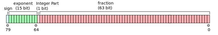
std::string GetLongDoubleBitsNice(long double val)
{
std::string bits = GetBitSequence((unsigned char*)&val, 10);
char buf[192];
snprintf(buf, sizeof(buf), "%3.4f d = %s %s %s %s b", (double) val,
bits.substr(0,1).c_str(), // sign bit
bits.substr(1,15).c_str(), // 15-bit exponent
bits.substr(16,1).c_str(), // integer bit
bits.substr(17,63).c_str()); // 63-bit mantissa
return std::string(buf);
}
int main(int argc, char** argv)
{
double Dlarge = 1.0;
double Dsmall = 1.0 / (double)(1ull << 53);
long double LDlarge = 1.0;
long double LDsmall = 1.0 / (long double)(1ull << 53);
std::cout << "sizeof(double) = " << sizeof(double) << std::endl;
std::cout << "sizeof(long double) = " << sizeof(long double) << std::endl;
std::cout << GetDoubleBitsNice(Dlarge) << std::endl;
std::cout << GetDoubleBitsNice(Dsmall) << std::endl;
std::cout << GetDoubleBitsNice(Dlarge + Dsmall + Dsmall + Dsmall + Dsmall
+ Dsmall + Dsmall + Dsmall + Dsmall
+ Dsmall + Dsmall + Dsmall + Dsmall
+ Dsmall + Dsmall + Dsmall + Dsmall) << std::endl;
std::cout << GetLongDoubleBitsNice(LDlarge) << std::endl;
std::cout << GetLongDoubleBitsNice(LDsmall) << std::endl;
std::cout << GetLongDoubleBitsNice(LDlarge + LDsmall) << std::endl;
return 0;
}As mentioned, on x64 architectures the classic x87 FPU is essentially replaced by the more modern SSE2 instruction set. However, using the compiler option g++ -mfpmath=387 LDtest.cpp enforces the usage of the classic x87 FPU with its 80-bit internal registers. The resulting output of the x87 FPU therefore shows a similar result as our float example in C# did before:
sizeof(double) = 8
sizeof(long double) = 16
1.0000 d  =  0 01111111111 0000000000000000000000000000000000000000000000000000 b   // 1.0
0.0000 d  =  0 01111001010 0000000000000000000000000000000000000000000000000000 b   // 2^(-53)
1.0000 d  =  0 01111111111 0000000000000000000000000000000000000000000000001000 b   // sum
1.0000 d  =  0 011111111111111 1 000000000000000000000000000000000000000000000000000000000000000 b
0.0000 d  =  0 011111111001010 1 000000000000000000000000000000000000000000000000000000000000000 b
1.0000 d  =  0 011111111111111 1 000000000000000000000000000000000000000000000000000010000000000 b
The important line is the third one: just like we discussed for the C# example, the intermediate computations leading to the result are being kept within the x87 FPU. The fact that we find a non-zero mantissa clearly shows, that more than the shown 52 bits of the mantissa are actually available for the (intermediate) computations. Compare this to the result that is produced using g++ -mfpmath=sse LDtest.cpp, which utilizes the SSE extension with true 64-bit double-precision variables:
sizeof(double) = 8
sizeof(long double) = 16
1.0000 d  =  0 01111111111 0000000000000000000000000000000000000000000000000000 b   // 1.0
0.0000 d  =  0 01111001010 0000000000000000000000000000000000000000000000000000 b   // 2^(-53)
1.0000 d  =  0 01111111111 0000000000000000000000000000000000000000000000000000 b   // sum
1.0000 d  =  0 011111111111111 1 000000000000000000000000000000000000000000000000000000000000000 b
0.0000 d  =  0 011111111001010 1 000000000000000000000000000000000000000000000000000000000000000 b
1.0000 d  =  0 011111111111111 1 000000000000000000000000000000000000000000000000000010000000000 b
As expected, the 52-bit mantissa in the third line here is zero since the intermediate computations have been carried out using 64-bit floating-point variables as well. It is the same result that we found using the 64-bit double type in the earlier C# code.
In the end, all of this is an interesting observation of the somewhat surprising effects of compiler options and different implementations of the floating-point run-time engine that is being used by the compiler. However, it does not really help us much from the practical point of view. The 80-bit extended precision variables are only accessible from certain compilers and are not even available in the .NET framework. Nevertheless, it is always good to know stuff in detail. At least now we have a good understanding of the origin and effect of a loss of significance in floating-point operations.
Handling a loss of significance
The loss of precision is a fundamental property of floating-point variables and mathematical operations, which conceptually are designed to be a practical compromise between numerical precision and limited memory capacity. Whatever we are going to do, this effect will always be present. The goal should therefore be to accept the issue and consider certain best practices to minimize the effects.
Kahan summation formula
As we have seen in much detail, the loss of precision essentially becomes important when we are adding numbers of significantly different magnitude, i.e. where the exponents are significantly distanced such that the mantissa has to be shifted quite a lot for a proper alignment. Considering that floating-point numbers are well-suited to keep track of small numbers (as well as large numbers), one approach is to simply keep track of all the small errors that arise in individual summations and aggregate those errors in a separate variable, where it can grow on its own and has the full mantissa available for error-tracking. This approach is sometimes called compensated summation and often attributed to William Kahan, one of the main x87 FPU designers and a pioneer of floating-point numeric analysis.
However, it is important to know that the Kahan summation formula is only useful when a lot of additions (at least two) are being performed. Obviously, it cannot extend the available precision of a given data type. The idea is to accumulate small errors that may grow to be big enough, such that they can be re-included to the sum. A prime example is our earlier loop of 16 additions of \(2^{-53}\) to 1.0 using double variables: each addition on its own produces the minute error \(2^{-53}\) in the sum, which is lost due to the limits of the data type. However, accumulating 16 additions of this error lets it grow to \(2^{-49}\) and this value can easily be hold by the double data format. Expanding on our earlier C# example, we can compare the plain summation to the Kahan summation formula:
public static float PlainSummation(float[] vals)
{
    float sum = 0.0f;
    foreach (float number in vals)
        sum += number;
    return sum;
}

public static float KahanSummation(float[] vals)
{
    float sum = 0.0f;
    float compensation = 0.0f;
    foreach (float number in vals)
    {
        float tmp_num = number - compensation;
        float tmp_sum = sum + tmp_num;

        compensation = (tmp_sum - sum) - tmp_num;
        sum = tmp_sum;
    }
    return sum;
}

static void Main(string[] args)
{
    float Flarge = 1.0f;
    float Fsmall = 1.0f / (float)(1 << 24);
    float[] FsmallArr = new float[17] { Flarge, Fsmall, Fsmall, Fsmall, Fsmall,
                                                Fsmall, Fsmall, Fsmall, Fsmall,
                                                Fsmall, Fsmall, Fsmall, Fsmall,
                                                Fsmall, Fsmall, Fsmall, Fsmall };

    float Fsum = PlainSummation(FsmallArr);
    Console.WriteLine(GetFloatBitsNice(Fsum));

    Fsum = KahanSummation(FsmallArr);
    Console.WriteLine(GetFloatBitsNice(Fsum));
}
If we run this piece of code, it produces the following result:
1.0000 d  =  0 01111111 00000000000000000000000 b    // plain summation result
1.0000 d  =  0 01111111 00000000000000000001000 b    // Kahan summation result
The first line is exactly the result, that we generated earlier in the Fsum += Fsmall loop and shows the effect of a repeated loss of significance in the addition.4 The Kahan summation formula, on the other hand, gives the correct result since the repeated correction term summarizes to the expected value \(2^{-20}\). We can repeat the same experiment using double variables and we will find the same effect. Considering that the .NET run-time limits the floating-point precision to 64-bit, as we have analyzed before, this is a very profound finding: if deemed necessary, we can use the Kahan compensated summation to minimize the loss of significance effect. In particular, an important benefit of the Kahan summation formula is the independence of the precision on the number of accumulated numbers, i.e. the loss of significance will always only be limited by the precision of the floating-point data type and not the number of summations.
One important aspect to consider in the usage of the Kahan summation formula is the effect of the optimizer: for example, in the assignment of the compensation value we have (tmp_sum - sum) - tmp_num, which simply reduces to sum for obvious algebraic reasons. Put together, all the computations are redundant and can be eliminated in theory, since we are just measuring the numeric errors of the computation. It is therefore crucial to actually test the results of a Kahan summation formula implementation in a given programming language and ensure that certain optimizer settings do not silently deactivate the compensation.
In the end, the usage of the Kahan summation formula is also a clear trade-off between precision and performance: Instead of a single addition for each element, the compensated summation requires 4 summations and 4 variable assignments, which (due to processor architectures and caches etc.) will result in a 4-8 times performance degradation. In other words, the loss of significance compensation is rather expensive to use in practice. Furthermore, it is only useful in a context were more than two floating-point numbers are added, otherwise the compensation will be truncated by the limits of the data type just the same as the regular addition. Note that in the examples that we discussed so far, we were considering rather extreme cases, where the loss of significance is shown in its most dramatic form.
Arbitrary precision floating-point numbers
Another possibility to increase numeric precision is to move away from fixed-width floating-point numbers altogether. As we have seen in the beginning of this discussion, the concept of floating-point numbers essentially just captures the scientific notation \((-1)^\sigma \cdot m \cdot 10^{e}\) and therefore leads to a variety of implementations. The focus on 32-bit single precision and 64-bit double precision floating-point numbers is not singled out by any conceptual benefits. Those two data formats have just appeared “naturally” on computers in the context of power-2-wide data sizes (16, 32, 64, 128, …), and subsequently led to high-performance hardware implementations, e.g. the x87 FPU and subsequent SSE extensions.
If the requirements for precision are important enough, one can always go back to a software implementation and chose a non-standard size for the floating-point number memory allocation, which can significantly increase the size of the mantissa or exponent (depending on application). The GNU multiple precision arithmetic library (called GMP for short) is a prominent and well-maintained implementation of such a general purpose software library for arbitrary precision arithmetic for integers and floating-point numbers. Using this emulation, the precision limit is essentially defined by the available memory of the machine. However, for obvious reasons, such a software emulation of the floating-point arithmetic comes at significant costs in terms of performance, which is several orders of magnitude slower compared to the hardware-accelerated standard data types float and double. As usual, we have a trade-off between precision and performance that has to be weighted for the problem at hand.
Overview of results and a best practice guide
As we reach the end of this discussion, it is useful to summarize all the findings regarding the loss of significance issue again. For everyday applications the following two best practices can always be followed without significant convenience issues or performance penalties:
- Use 64-bit
doubleinstead 32-bitfloatvariables. Aside from the doubled memory requirements, there is no performance difference on modern CPUs from use of the double-precision variables.5 The data from the variables will be converted to an internal format in any case, which will usually be a normalized data format corresponding to the widest data type that can be handled by the hardware: 80-bit extended precision on classic x87 FPUs or 64-bit double precision of modern SSE/SSE2 extensions found in the x64 CPU architecture. - Limit use of temporary variables. This recommendation is somewhat at odds with common best practices regarding readability and code maintainability. However, our findings on keeping computations on the floating-point stack clearly show, that eliminating temporary variables can increase the computational precision if the used variable data type is smaller than the internal normalized data format of the floating-point engine. Therefore this suggestion technically only applies to the use of 32-bit
floatvariables in the .NET framework or 64-bitdoublevariables on native code that may be executed on the x87 FPU. Aside from the loss of precision issue, the use of temporary variables may also incur additional memory movement instructions, which can be relatively slow as well. A decent optimizer should be able to handle those, but there are no guarantees.
Certain high-precision applications may require more sophisticated steps that go beyond what those “tricks” can provide:
- Use compensated Kahan summation. In case that more than two floating-point numbers are being added, one can benefit from the Kahan summation algorithm, which accumulates small errors of each addition in order to minimize the loss of significance effect. However, as discussed, the performance hit comes at a factor of 4–8 depending on the hardware specifics.
- Use arbitrary precision variables. When everything else does not suffice, one has to go the step to arbitrary precision floating-point numbers, which are emulated using the integer logic functions of the CPU. The performance hit compared to hardware-accelerated floating-point arithmetic will be rather dramatic (at least a factor of around 50, usually significantly more) and depends entirely on the chosen specifics of the emulated data format.
What was left out
Aside from the issue of a loss of significance, we entirely ignored various other aspects of floating-point numbers. For example, the issue of rounding is similarly important and related to the problem discussed here. From a certain perspective, what we have covered here is a special case of rounding (“truncating”), but the general story is much more involved. Furthermore, while we have focused on additions, the loss of significance is also present in other mathematical operations like multiplication etc. However, there are no “simple remedies” like the compensated summation available for those issues.
As a follow-up to this text I can highly recommend reading the technical paper “What every computer scientist should know about floating-point numbers“, which dives deeply into the issue of floating-point rounding and numerical analysis.
-
Modern desktop and notebook CPUs today always have an FPU, but certain low-power or low-end embedded micro-controllers may not. In such cases one has to emulate the floating-point arithmetic using software that exclusively uses the integer arithmetic logic units (ALUs) of the CPU. A free, high-quality implementation is the Berkeley SoftFloat package, which is maintained by John Hauser. It it quite educating to follow the necessary steps—and especially the special cases one has to consider—for a simple operation like the addition of two floating-point numbers in full detail. ↩
-
One early example of a floating-point unit was the Scientific Instruction Set feature, which was available as an option on the famous IBM System/360 mainframe computers of the 1960s and early 70s. It could operate both on 32-bit and 64-bit floating-point numbers and emulate 128-bit operations as well. Those implementations used the IBM Floating Point Architecture, which was superseded by the IEEE-754 standard about 20 years later in 1985. The main difference between the IBM design and the IEEE standard was a stronger focus on the number precision, i.e. a longer mantissa and a smaller exponent. ↩
-
Multiplication in base-2 is much simpler than in base-10: Whereas the single-digit multiplication table in base-10 has 100 entries, in base-2 we only have 4 entries: \(0 \cdot 0 = 0\), \(1 \cdot 0 = 0\), \(0 \cdot 1 = 0\) and \(1 \cdot 1 = 1\) and this corresponds exactly to the input-output table of the AND logic gate. Keeping this in mind, the multiplication of two binary numbers is performed in the same way, in which one would multiply two decimal numbers by hand: one of the numbers is basically shifted from least to most significant digit of the other number (i.e. effectively multiplied by powers of 10) and only multiplied with the relevant single digit. Then the intermediate terms are just summed up. Therefore, once we have the circuitry to add two binary numbers and the AND logic gate, we can easily do binary multiplications as well. ↩
-
In a release build where aggressive optimization is turned on, we may actually find the correct result from the plain summation using
floatvariables. Since the optimizer will attempt to minimize unnecessary memory access, the intermediate sum insum += numberfrom each loop iteration will remain on the top of the floating-point stack, where it effectively utilizes the double precision mantissa. Switching todoublevariables andFsmall = 1.0 / (double)((ulong)1 << 53), the effect of the compensated Kahan summation becomes apparent as well. ↩ -
The usage of double-precision vs. single-precision floating-point numbers has a significant performance impact on massively parallelized computations that run on modern graphics processors (GPUs). Since typical 3d graphics applications can be well handled using single precision floating-point numbers, the hardware implementations focus on the smaller data type. At the point of writing, the performance difference between single and double precision still comes around to a factor of about 3–4 even on hardware targeted towards scientific computing, i.e. double precision applications. However, altogether one has to deal with a whole bunch of other issues in this domain, and in the text we are exclusively dealing with floating-point numerics on standard desktop computers and CPUs. ↩